Selecting the right species for a planting project can be complex, requiring both ecological knowledge and practical considerations to ensure successful growth and alignment with project goals. In this tutorial, we’ll walk through an example using Finca Caimito, a real planting site in northern Andalucía near Castilla-La Mancha, to demonstrate how specific tools can guide informed species selection.
For Finca Caimito, the landowners aimed to cultivate a diverse array of species using the Miyawaki method, which fosters rapid biodiversity development and encourages natural seed dispersal by animals to support passive ecological restoration in surrounding areas. Understanding this objective, we’ll use the site’s KML file to select a preliminary group of at least 20 species that align with these goals.
Step 1: Use the Map of the Natural Vegetation of Europe, climate data and IPCC projections to select reference ecosystems
First, download the desktop app Map of the Natural Vegetation of Europe (MNVE from now on) and a KML copy of the MNVE. Using both resources will allow you to tell precisely in which map unit(s) our reforestation site is located.
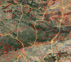
Open the KML copy of the MNVE and the planting site KML with any GIS tool (i.e. Google Earth). Once you open the KML files, you will see something like this:
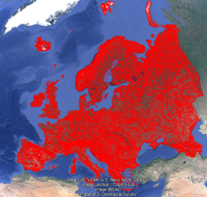
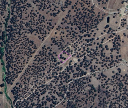
Open the MNVE app and select the “Map” tab at the top. Use the “Zoom in” button from the interface to approach the area of interest. Comparing the shapes on the MNVE and the MVNE copy in Google Earth, click on the point where you would locate the restoration site in the MNVE, using the “layer info” button from the toolbar (Important: the map is on a continental scale, so the accuracy is limited. Sometimes you can judge the true limits of vegetation types by looking at the features of the satellite images (mountains, flood plains) and adjust the selection accordingly). The map unit where our site is located is now highlighted in red:
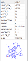
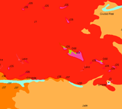
Identify the code of the selected layer (in this case, J1), and type it in the search panel on the left.
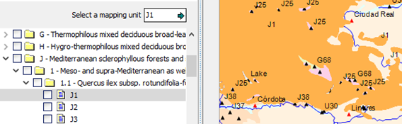
Select the “Text mapping units” tab on the top. There you have plenty of information regarding the selected vegetation formation:

But before looking at the species, let’s have a look at the climate. In a changing climate, we should check whether the potential vegetation according to the MNVE is compatible with future scenarios. Let’s see what the climate may look like in the future (2060s) in this area with the help of some tools. For that, we can use this template to see the interactive climate atlas of our region of interest (in our case Spain in the Iberian Peninsula). Once in the viewer, we can zoom into to the area of interest, select the exact area or coordinates by clicking, and find the relevant climate data.
For our example, we see that the mean annual temperature in the area was around 15.1ºC during the 1971-2000 period, and the mean annual precipitation, around 640 mm.
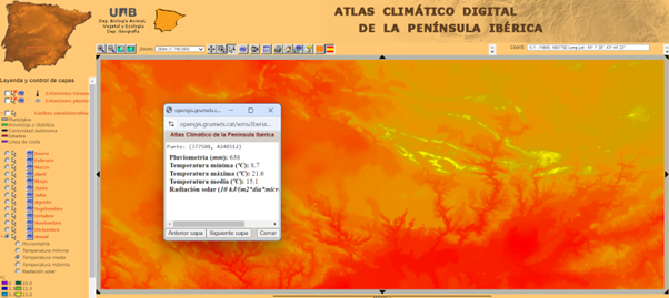
Now, going back to the template, we can take a look at the projected changes for mid-century (second group of selected comparisons), for the mean annual temperatureand precipitation, in that area. Using the 'Point Information' option in the toolkit on the right in the Interactive IPCC Atlas, we observe that, by mid-century under the RCP 2.6 scenario, the mean annual temperature is projected to increase by around 2.2 ºC, and mean annual precipitation is expected to decrease by around 7.7%, relative to the 1971-2000 period.
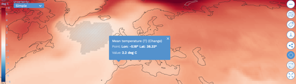
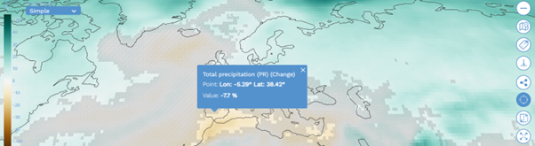
Now, let’s calculate the projected values for mean annual temperature and precipitation and assess the suitability of the vegetation formation.
You can use this tool (the “Simple” sheet) to annotate the values and calculate the projected values. You can use the “Complete” sheet for a more detailed evaluation, but more inputs will be required (monthly and seasonal values). For a rough estimate, we have enough with just mean annual temperature and precipitation. According to the reference data and the IPCC projections, we can expect a mean annual temperature of around 17.3ºC and a mean annual precipitation of around 590 mm at the site by mid-century. This is at the upper limit of the temperature range of our vegetation formation, and still within the annual precipitation range.
Now we will search for another vegetation formation that thrives in similar soil types but in warmer environments which are more compatible with the projected climate, and base the selection of species on both vegetation formations.
The vegetation formation J1 grows on siliceous rocks, and thus we should look for another formation that thrives in warmer conditions but also on siliceous rocks.
Such is the case of the vegetation formation J37:
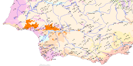

Now, let’s see the details regarding species composition and ecological and geographical variants and combine the species from both vegetation formations according to site characteristics.
For that, it can be helpful to ask ourselves the following questions:
→ Is the terrain flat, a sun-facing slope, a shady slope, or a combination of these?
In our case, Flat. Hence, we can expect high irradiation but likely a relatively deep or stable soil as well.
→ Are there any water bodies on the site?No. If there were, we could look at which are typical riparian communities accompanying these vegetation formations.
→ Does the soil show any signs of degradation (bare soil, gullies, compacted)?Some. There seem to be some areas with bare or compacted soil, perhaps due to the presence of cattle, but there are areas that seem to have relatively low impact. So we should explicitly plan the distribution of the species accordingly. We should reserve the most degraded areas for pioneer species, and plant the other species in normal conditions or partially to fully under the shade of existing trees according to their needs.
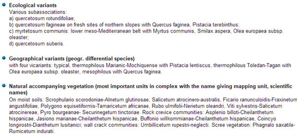

From J1 (see images above), we include all the dominant and frequent species listed above except Asparagus acutifolius, which often persists in degraded areas and likely does not need to be planted (however, we should be familiar with the site and actually know what species are already there, their approximate abundance and whether they are regenerating properly). Quercus ilex is already present (in this case we can tell from the satellite images), but in quite low density. We could leave it on the list to assist regeneration if needed. We incorporate Myrtus communis and Olea europaea subsp. oleaster (Smilax aspera is a vine) which are common on the warmest sites in which this formation occurs. We exclude Pistacia terebinthus because, according to the MNVE, it prefers northern slopes in the given climate. Quercus faginea is likely not suitable for the projected climate, and is therefore excluded.


From J37 (see images above), we include all species not included in J1. This leaves the following species:
Tree species (4): Quercus ilex subsp. rotundifolia, Pyrus bourgaeana, Quercus suber, Ceratonia siliqua.
Shrub species (15): Daphne gnidium, Jasminum fruticans, Quercus coccifera, Pistacia lentiscus, Retama sphaerocarpa, Genista hirsuta, Lavandula stoechas subsp. sampaiana, Phillyrea angustifolia, Cystus multiflorus, Myrtus communis, Olea europaea subsp. oleaster, Chamaerops humilis, Osyris lanceolata, Rhamnus lycioides subsp. oleoides, Arbutus unedo.
Let’s look for some additional species.
Step 2: Use the internal species listing tool to select additional species
Now, we can open the species listing tool developed by Life Terra based on EUFORGEN species distribution maps and select the site location. The app will show us a list of native tree and large shrub species whose distribution ranges overlap in this location
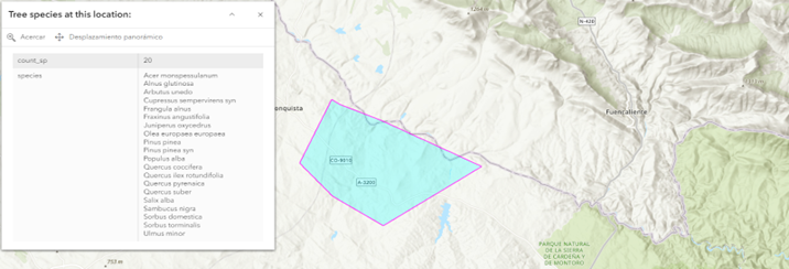
Here, we can look for species not included in our previous list to increase richness. However, not all the species listed in the app are necessarily suitable for our site. This is because the resolution of the distribution maps is coarse and thus they are particularly prone to error when species are near the limit of their range, and also in the case of species which have special soil requirements (e.g., riparian species). Hence, it is necessary to pay attention to species’ autecology when selecting species from this list. Here are some tools that can be used to filter the species according to their autecology:
Árboles Ibéricos, ArbolApp, Herbario de Jaca (for the Iberian Peninsula, but also useful for the Mediterranean region in general; ArbolApp is also available in english)
In our example, see below the observed species for the area of interest:
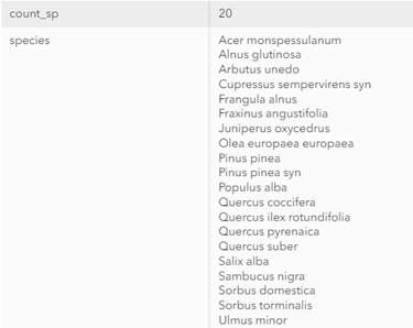
Based on the list, Alnus glutinosa, Fraxinus angustifolia, Populus alba, Salix alba and Ulmus minor we classified as unsuitable because they are riparian species under Mediterranean climate. Frangula alnus, Quercus pyrenaica, Sambucus nigra, Sorbus domestica and Sorbus torminalis are also classified as unsuitable because they require cooler and more humid conditions than those provided by the site. Acer monspessulanum will likely not tolerate the projected climate.
Despite its introduction to the Iberian Peninsula millennia ago and its suitability to current and projected site conditions, Cupressus sempervirens is excluded due to its allelopathic effects, which impede understory growth. Juniperus oxycedrus and Pinus pinea are suitable and added to the species list (but the latter should be planted in small numbers, because its dense canopy limits understory growth).
After that we end up with a solid list of suitable species (in our example, we got 21 suitable species). Next steps should include evaluating practical considerations like nursery availability, cost, and alignment with the goals of the landowner and those responsible for maintaining the plantation. This alignment is crucial to ensure that the selected species meet both ecological and management needs, enhancing the long-term success and sustainability of the project.
Good Planting!
If you have any questions or suggestions for improvement, or know of other resources that could be helpful, please don't hesitate to let us know.